ClickHouse outcompresses Parquet: Surprises from our migration

I'm not affiliated with ClickHouse, Inc. We use the free, open-source version.

I have been leading an initiative to migrate our core IoT datasets, consisting of trillions of rows, to a self-hosted ClickHouse cluster on Hetzner bare metal. While ClickHouse is famously fast, we learned that it is also excellent at compressing data, which is highly relevant at our scale. This post explores the tricks we used to noticeably outperform our previous optimized Parquet setup on this front.

Schema

The schema we'll be working with represents vehicle GPS pings. A vehicle sends a latitude, longitude ping at time_sent, while time_received is the time at which it reaches our servers. Pings from the same vehicle's session send the same (anonymized) session_id. A row also contains some additional data, like speed and heading.

• session_id: string
• latitude: double
• longitude: double
• time_sent: timestamp, second precision
• time_received: timestamp, second precision
• speed: uint8
• heading: uint16
• hdop: uint16

We ingest over a trillion of such rows per year, or over 50k rows per second. Therefore, it's definitely worth it to try to optimize the storage a bit!

Parquet

Parquet is a popular columnar file format. Columnar means that data is stored column-by-column, instead of row-by-row. Although this makes the retrieval of a single row slower and more difficult, it comes with clear advantages. The most relevant one for us is that, when paired with a good sort order, it is significantly easier to compress subsequent values of a column than trying to compress mixed data across an entire row.

Since we're not that interested in retrieving single rows, this makes Parquet a solid choice for us. It is also what we were using before we started migrating to ClickHouse. Here's the original Parquet schema:

int64   s2_cell_id     INTEGER(64, false);       -- PLAIN
binary  session_id     STRING;                   -- PLAIN
int32   latitude_e6    INTEGER(32, true);        -- DELTA_BINARY_PACKED
int32   longitude_e6   INTEGER(32, true);        -- DELTA_BINARY_PACKED
int64   time_sent      TIMESTAMP(MILLIS, true);  -- DELTA_BINARY_PACKED
int64   time_received  TIMESTAMP(MILLIS, true);  -- DELTA_BINARY_PACKED
int32   speed          INTEGER(8, false);        -- PLAIN
int32   heading        INTEGER(16, false);       -- PLAIN
int32   hdop           INTEGER(16, false);       -- PLAIN

The first type shows the physical type, the second type shows the logical type, and the comment shows the encoding used. We used a couple tricks to get the compressed size as low as possible, so let's take a look.

Sort order

When using a columnar format, the sort order is very important, as it determines the order in which values are compressed. If subsequent values follow a predictable pattern, they are much easier to compress.

If we were purely interested in compressed size, a simple and good sort order would be (session_id, time_sent). This groups pings from the same vehicle together, maximizing the compression ratio. It also makes it easy to retrieve an entire session. However, if you want to retrieve all pings within a certain area (a geospatial query), you have to do a full scan over the data, as the relevant pings will be dispersed over the entire file. At our scale, that would mean these types of queries would be too slow to execute for most use cases. This was not acceptable for us. Therefore, we introduced a new column: s2_cell_id.

S2 cells divide the earth's surface into rectangular¹ cells, such that cells which are close to each other in space tend to have numerically close IDs. Essentially, we're trying to map a 2D space (the earth's surface) onto a 1D line (numeric IDs), while preserving the concept of proximity as best as possible. This is done by using a Hilbert space-filling curve. S2 cells are hierarchical: Lower levels have larger cells, higher levels have smaller cells.

If we calculate the S2 cell at a given level for every GPS point (this is computationally cheap), and then change our sort order to (s2_cell_id, session_id, time_sent), we can enable fast geospatial queries over the data, while maintaining good compression. Lower S2 cell levels (larger cells) produce longer contiguous runs of points for a given session_id, improving compression, but making small-area geospatial lookups read more superfluous data. On the other hand, higher S2 cell levels (smaller cells) make it possible to skip data more granularly, making small geospatial lookups faster, but shorten average runs from the same session_id, worsening compression.

In our custom Parquet writer, we first clustered data into row groups of ~1M rows based on their level 11 S2 cells, and then sorted on (session_id, time_sent) within each individual row group. This makes it so that each row group "owns" a piece of the surface, with areas where data density is higher resulting in smaller row groups than areas with lower data density. Geospatial queries now only have to retrieve row groups whose areas overlap with the queried area. Here's an example of an hour of data from a provider that mostly sends data from the Netherlands:

In ClickHouse, we went for a simpler solution. We settled on level 8 S2 cells, and just sorted on (s2_cell_id, session_id, time_sent). To keep comparisons fair, we'll use this same sort scheme for Parquet in the results below as well, instead of our custom solution.

Latitude and longitude as integers

Double-precision can store lat/lon pairs to nanometer precision, but of course, the precision of the incoming data is many orders of magnitude worse, and we don't care about this level of precision anyway. Storing lat/lon as doubles leads to noisy bits in the mantissa that are difficult to compress. Instead, we can multiply latitude and longitude by 1e6, round it, and store the result in a 32-bit integer. The maximum longitude is ±180°, so multiplying that by 1e6 gives 180 million, which comfortably fits inside an int32 (which has limits of roughly ±2.1 billion). As the maximum latitude is ±90°, both lat and lon are always guaranteed to fit in an int32.

With this representation, we halve the uncompressed size of our data, and we drop down to centimeter precision (max error of ~6 cm for one lat/lon point). This is still more than good enough for what we need to do. By lowering the precision, we get rid of a lot of noise, and the resulting data compresses much better.

Parquet encodings

It is well known that Parquet lets you compress column data using compression codecs like Snappy or ZSTD. You might also know that you can use dictionary encoding (RLE_DICTIONARY) to achieve high compression ratios on low-cardinality columns. What is less known, and less utilized, however, is that the Parquet standard supports more encodings than just PLAIN or RLE_DICTIONARY. Support for these other encodings is mixed in practice. Although most readers can read columns written with these encodings, many are unable to write them.

However, DELTA_BINARY_PACKED turned out to be quite beneficial for some of our columns, so we found a writer that did support it. The encoding works by calculating the delta between subsequent values in the column, and then applying a binary packing strategy that is most effective when deltas are small. The result can then be fed into a general purpose compression codec. We use ZSTD, as it provides a great balance between compression ratio and (de)compression speed.

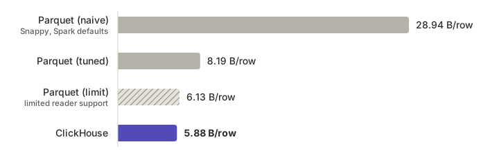
After applying all the tricks above, we end up at around 8.2 bytes per row compressed. Note that a naive implementation where we limit ourselves to Snappy compression and the PLAIN and RLE_DICTIONARY encodings (the default Spark settings) gets around 28.9 bytes per row. And if you mess up the sort order and sort on time_received instead, you end up at around 59.4 bytes per row. Therefore, I think it's fair to say that we've pushed Parquet reasonably hard.

Pushing Parquet to the limit

But if we're willing to sacrifice compatibility and quality of life, we can push Parquet even further. First off, we've been storing time_sent and time_received in millisecond precision timestamps, despite them only having second precision. Why? Because Parquet simply does not support second precision timestamps. So let's make two changes: We'll manually encode and store time_sent as an int32, and we'll drop time_received, instead storing received_latency, where time_received = time_sent + received_latency. It'll be the responsibility of the reader to reconstruct this column.

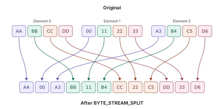
Secondly, the Parquet standard was recently updated to allow using the BYTE_STREAM_SPLIT encoding for integer types, while it was only supported for floating point types before. This encoding works by rearranging the bytes of the values as shown below:

By itself, it does not reduce the data size, but when paired with ZSTD, the results significantly outperform DELTA_BINARY_PACKED on our biggest columns. Why does DELTA_BINARY_PACKED perform poorly by comparison? I'm not 100% sure, but I think the bit packing can straddle different values over byte boundaries, messing with ZSTD, which looks for repeating patterns at the byte level.

Unfortunately, reading integer columns encoded with BYTE_STREAM_SPLIT is a new and relatively unsupported feature. Major readers like DuckDB and Polars will simply throw an error when encountering this.

With these changes, Parquet hits about 6.1 bytes per row. But realistically, the limitations with this approach are probably a dealbreaker in most cases. Can ClickHouse still do better than this? Yes!

ClickHouse

ClickHouse is an OLAP database. ClickHouse, Inc. sells a managed version of ClickHouse called ClickHouse Cloud, but we chose to self-host the open source version of ClickHouse on Hetzner bare-metal instead. ClickHouse's main table engine, the MergeTree, also stores data in a columnar fashion, just like Parquet. Each node in the cluster stores its data directly on its own NVMe SSDs. This makes queries ridiculously fast. However, SSDs are quite a bit more expensive than hard drives (like S3 uses), especially with recent AI-related price hikes. That makes optimizing the compressed size per row even more relevant than before.

Here's the original Parquet schema, ported to ClickHouse:

CREATE TABLE gps
(
    s2_cell_id        UInt64           CODEC(ZSTD(3)),
    session_id        String           CODEC(ZSTD(3)),
    latitude_e6       Int32            CODEC(DoubleDelta),
    longitude_e6      Int32            CODEC(DoubleDelta),
    time_sent         DateTime('UTC')  CODEC(DoubleDelta, ZSTD(3)),
    received_latency  Int32            CODEC(T64, ZSTD(3)),
    time_received     DateTime('UTC')  ALIAS time_sent + received_latency,
    speed             UInt8            CODEC(Delta, ZSTD(3)),
    heading           UInt16           CODEC(ZSTD(3)),
    hdop              UInt16           CODEC(T64, ZSTD(3))
)
ENGINE = MergeTree
ORDER BY (s2_cell_id, session_id, time_sent)

Incredibly, this ClickHouse port reaches about 5.9 compressed bytes per row, despite the fact that we're using a much lower ZSTD level (3 for ClickHouse vs 11 for Parquet)². How is this possible? Let's look at a comparison of the most important columns:

DBP = DELTA_BINARY_PACKED / BSS = BYTE_STREAM_SPLIT / DD = DoubleDelta

It seems like DoubleDelta outperforms both Parquet encodings. How does it work?

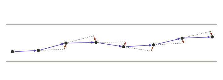
Imagine a vehicle is driving along a straight road. Delta stores the difference between two consecutive points (blue vectors). DoubleDelta stores the difference between two consecutive deltas (red vectors). Another way to think about it is that DoubleDelta "predicts" the next point will be at the same delta offset as the previous point's delta, and then "corrects" itself with a second offset. In this case, it is clear that the red vectors are smaller than the blue vectors, which can intuitively explain why it compresses better.

Of course, this encoding is most effective when vehicles are driving along a straight road for long periods of time at a constant speed. Luckily, a majority of our data is from highways, so that checks out! Unfortunately, Parquet has no encoding like this³, so this is a clear advantage for ClickHouse.

Ease of use

The ClickHouse schema gets a better byte per row result than the best Parquet schema, while maintaining good quality of life for data consumers. The DateTime type is a second precision timestamp, physically stored as a 32-bit integer. This is the exact type we needed from Parquet, but which it didn't have. So now readers can natively use whichever timestamp functions they want.

Also, with time_received being stored as an ALIAS, readers can query it directly, and ClickHouse will transparently compute the values at query time by adding the time_sent and received_latency columns.

Results

When both Parquet and ClickHouse are tuned for maximum compression, ClickHouse comes out on top, at least for this dataset:

Assuming a dataset size of 5 trillion rows (a bit more than 3 years of data), this would be the cost of storing each of these on S3:

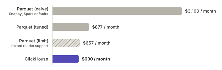
S3 Standard in us-east-1 at $0.023 per GB-month

Assuming we wanted to store the entire dataset on NVMe SSDs, this is how much each solution would cost per month. We assume each row is stored on three replicas, and use current Hetzner prices for the node type we're currently using in our production ClickHouse cluster.

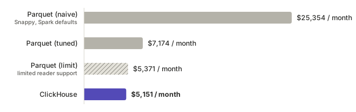
Hetzner EX63 at €802 (≈ $897) per month for 4 × 3.84 TB NVMe with 3× replication

1. These are technically spherical quadrilaterals. But in this case, ignoring the scary math words and pretending they're just rectangles works remarkably well. ↩
2. Using a lower ZSTD level in ClickHouse as opposed to Parquet is desirable, as ClickHouse has write amplification due to MergeTree merges. Using ZSTD(11) drops us down to about 5.75 bytes/row. ↩
3. By the way, DoubleDelta isn't quite the same as just doing Delta twice, as it also does a bit packing step at the end, just like DELTA_BINARY_PACKED. And just like with that encoding, this might screw with ZSTD. On the latitude and longitude columns, appending ZSTD(3) after DoubleDelta doesn't improve compressed size at all. On the time_sent column, ZSTD(3) can still noticeably improve the result from DoubleDelta. But on ZSTD levels 15 and up, Delta, ZSTD starts outperforming DoubleDelta, ZSTD, potentially because the bit packing finally starts to hurt? I don't know, this is quite obscure stuff. In any case, level 15 is too slow to reasonably use in production anyway. ↩